Scientific and Engineering Libraries, Part 2

Weeks 12 and 13 are about using external scientific and engineering libraries that are not inside core Python, but are popular enough that we should learn them too.

Pandas

Pandas is a Python library for easy and efficient numerical computation of table-like data. You can install it via either pip or conda with, for example the following command:

pip install pandas

We generally import pandas as "pd".

import pandas as pd

Assume that you have the following data:

columns = ['Name', 'Grade', 'Age']
data = [
    ['Jack', 40.2, 20],
    ['Amanda', 30.0, 25],
    ['Mary', 60.2, 19],
    ['John', 85.0, 30],
    ['Susan', 70.0, 28],
    ['Bill', 58.0, 28],
    ['Jill', 90.0, 27],
    ['Tom', 90.0, 24],
    ['Jerry', 72.0, 26],
    ['George', 79.0, 22],
    ['Elaine', 82.0, 23]
]

We can read this using pandas by converting it to a pandas.DataFrame:

data = pd.DataFrame(data=data, columns=columns)

Here's how it looks:

data

	Name	Grade	Age
0	Jack	40.2	20
1	Amanda	30.0	25
2	Mary	60.2	19
3	John	85.0	30
4	Susan	70.0	28
5	Bill	58.0	28
6	Jill	90.0	27
7	Tom	90.0	24
8	Jerry	72.0	26
9	George	79.0	22
10	Elaine	82.0	23

Pandas has a multitude of different reader and writer functions to read/write data from a different file format.

We can quickly save our data as a CSV file with .to_csv():

data.to_csv('my-data.csv', index=False)

And read it back using .read_csv():

data = pd.read_csv('my-data.csv')

Our data has three columns, and eleven students. We can access a column like this:

data['Grade']

0     40.2
1     30.0
2     60.2
3     85.0
4     70.0
5     58.0
6     90.0
7     90.0
8     72.0
9     79.0
10    82.0
Name: Grade, dtype: float64

If we want, we can also create "row labels" (i.e, an index), using the names of the students:

data = data.set_index('Name')

data

	Grade	Age
Name
Jack	40.2	20
Amanda	30.0	25
Mary	60.2	19
John	85.0	30
Susan	70.0	28
Bill	58.0	28
Jill	90.0	27
Tom	90.0	24
Jerry	72.0	26
George	79.0	22
Elaine	82.0	23

This way, we can access a student's information by providing their name as an index to the .loc[...] attribute:

data.loc['Amanda']

Grade    30.0
Age      25.0
Name: Amanda, dtype: float64

Instead of using .loc[...], we could also access a integer-specified "row" using the .iloc[...] attribute with a numeric index:

data.iloc[1]

Grade    30.0
Age      25.0
Name: Amanda, dtype: float64

data

	Grade	Age
Name
Jack	40.2	20
Amanda	30.0	25
Mary	60.2	19
John	85.0	30
Susan	70.0	28
Bill	58.0	28
Jill	90.0	27
Tom	90.0	24
Jerry	72.0	26
George	79.0	22
Elaine	82.0	23

We can access a specific grade, using the following syntax:

data.loc['Jack']['Grade']

np.float64(40.2)

data['Grade']['Jack']

np.float64(40.2)

data.loc['Jack', 'Grade']

np.float64(40.2)

Chained indexing

One trick to watch out for: when we want to change a value inside of a DataFrame, you should avoid using chained indexing.

If we try to change Jack's grade using this syntax, we get a warning:

data['Grade'].loc['Jack'] = 73

/var/folders/td/_xx1fpkj2njc79sp8fh8xlch0000gn/T/ipykernel_28405/2411893513.py:1: ChainedAssignmentError: A value is being set on a copy of a DataFrame or Series through chained assignment.
Such chained assignment never works to update the original DataFrame or Series, because the intermediate object on which we are setting values always behaves as a copy (due to Copy-on-Write).

Try using '.loc[row_indexer, col_indexer] = value' instead, to perform the assignment in a single step.

See the documentation for a more detailed explanation: https://pandas.pydata.org/pandas-docs/stable/user_guide/copy_on_write.html#chained-assignment
  data['Grade'].loc['Jack'] = 73

Pandas might still update the value for you (depending on the version of pandas), but this is not the solution.

The best practice is to do this instead, which will not produce a warning:

data.loc['Jack', 'Grade'] = 83

data

	Grade	Age
Name
Jack	83.0	20
Amanda	30.0	25
Mary	60.2	19
John	85.0	30
Susan	70.0	28
Bill	58.0	28
Jill	90.0	27
Tom	90.0	24
Jerry	72.0	26
George	79.0	22
Elaine	82.0	23

Pandas has some nice functions that are useful for getting quick statistics about your data:

For numeric data, .describe() will produce some general stats about the given columns:

data.describe()

	Grade	Age
count	11.000000	11.000000
mean	72.654545	24.727273
std	17.848045	3.495452
min	30.000000	19.000000
25%	65.100000	22.500000
50%	79.000000	25.000000
75%	84.000000	27.500000
max	90.000000	30.000000

For example, we see that the mean age is 24.72.

.sort_values(col) will reorder the data such that the rows are sorted from lowest-to-highest for that given category:

data.sort_values('Grade')

	Grade	Age
Name
Amanda	30.0	25
Bill	58.0	28
Mary	60.2	19
Susan	70.0	28
Jerry	72.0	26
George	79.0	22
Elaine	82.0	23
Jack	83.0	20
John	85.0	30
Jill	90.0	27
Tom	90.0	24

Using ascending=False will sort the values from largest to smallest:

data.sort_values('Age', ascending=False)

	Grade	Age
Name
John	85.0	30
Susan	70.0	28
Bill	58.0	28
Jill	90.0	27
Jerry	72.0	26
Amanda	30.0	25
Tom	90.0	24
Elaine	82.0	23
George	79.0	22
Jack	83.0	20
Mary	60.2	19

.value_counts() can help with counting the number of different values for a given field:

data.value_counts('Grade')

Grade
90.0    2
83.0    1
30.0    1
60.2    1
85.0    1
70.0    1
58.0    1
72.0    1
79.0    1
82.0    1
Name: count, dtype: int64

.nlargest(num, col) will give you the rows with the largest value for the given column:

data.nlargest(3, columns='Grade')

	Grade	Age
Name
Jill	90.0	27
Tom	90.0	24
John	85.0	30

Finally, .plot() will produce graphs of line plots of your data:

data.plot()

<Axes: xlabel='Name'>

data['Grade'].plot()

<Axes: xlabel='Name'>

As a final remark, if you ever wonder the internal datatype used to represent data in Pandas data, they are often stored as NumPy-compatible arrays:

data['Grade'].values

array([83. , 30. , 60.2, 85. , 70. , 58. , 90. , 90. , 72. , 79. , 82. ])

data.values

array([[83. , 20. ],
       [30. , 25. ],
       [60.2, 19. ],
       [85. , 30. ],
       [70. , 28. ],
       [58. , 28. ],
       [90. , 27. ],
       [90. , 24. ],
       [72. , 26. ],
       [79. , 22. ],
       [82. , 23. ]])

Matplotlib

Matplotlib is a widely-used library to produce plots and graphs of various forms in Python.

You can install it via

pip install matplotlib

import matplotlib.pyplot as plt

Let's go over the anatomy of a matplotlib graph, from the example in the textbook:

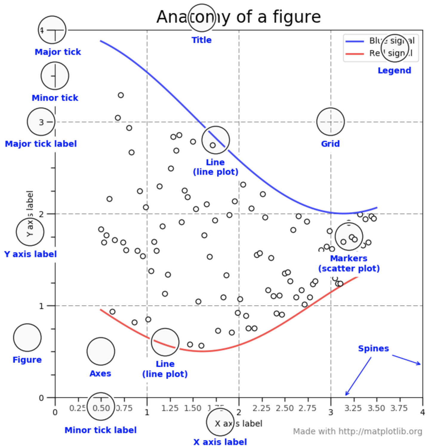
The figure above has several key features:

• It has a main title (title), x-axis title (xtitle) and a y-axis title (ytitle).
• It has two lines which have different colors and two labels that are shown in the little box (legend).
• The numeric values in the table are have their values shown using the numbers on the axes (the ticks).

Every part of the anatomical graph components are customizable in matplotlib.

Let's draw the simplest graph, using the pyplot API.

plt.plot(x_values, y_values) is for drawing a lineplot that passes through each pair of points given by x_values and y_values, which are either lists or NumPy arrays:

xs = list(range(10))
ys = [x**2 for x in xs]
plt.plot(xs, ys)

# Customizing the graph
plt.xlabel('x')
plt.ylabel('y')
plt.title('Graph of x ** 2')

Text(0.5, 1.0, 'Graph of x ** 2')

If we need to plot multiple lines into the same plot, we can just call plt.plot() multiple times.

The following example makes use of the OOP approach of using matplotlib, which is calling plt.subplots() to get fig and ax objects, and using the ax object to draw the graph.

Notice that most function calls using ax are the same, but some have .set_ as a prefix to the function call.

fig, ax = plt.subplots()

ax.plot([x**2 for x in range(1, 10)], label='$f(x) = x^2$')

# Display this with a gray color
ax.plot([x**3 for x in range(1, 10)], label='$f(x) = x^3$', c='tab:gray')


ax.set_xlabel('x')

# Show 10 ticks
ax.set_xticks(range(10))

# Display the legend
ax.legend()

# Add a grid
ax.grid()

# Display the y values in logarithmic scale
ax.set_yscale('log')

ax.set_title('Graph of polynomials')

Text(0.5, 1.0, 'Graph of polynomials')

We frequently need to draw multiple subplots inside a single plot, which is possible in the OOP style by giving row and column numbers to the plt.subplots() call to get multiple subplots, and then drawing each plot in its own plot:

# Plot x ** 2
fig, ax = plt.subplots(1, 2)  # 1 row, 2 columns of plots
ax[0].plot([x**2 for x in range(10)])
ax[0].set_xlabel('x')
ax[0].set_title('y = x ** 2')

# Plot x ** 3 on the second canvas
ax[1].plot([x**3 for x in range(10)])
ax[1].set_xlabel('x')
ax[1].set_title('y = x ** 3')

Text(0.5, 1.0, 'y = x ** 3')

This is also possible using the pyplot style. To make plt switch to one specific subplot, the plt.subplot(...) call should end with the currently-switched plot number.

# Draw x ** 2
plt.subplot(1, 2, 1) # 1 row, 2 columns of plots, switch to first plot
plt.plot([x**2 for x in range(10)])
plt.xlabel('x')
plt.title('y = x ** 2')

plt.subplot(1, 2, 2) # Same thing, but switch to second plot
plt.plot([x**3 for x in range(10)])
plt.xlabel('x')
plt.title('y = x ** 3')

Text(0.5, 1.0, 'y = x ** 3')