The volume of the n-ball

This is the second entry in the high-dimensional space blog series.

In the previous post, we were able to calculate the (hyper-)volume of the $4$-dimensional ball of radius $R$ as

\[V_{4}(R) = \frac{1}{2}\pi^2 R^{4}.\]

How do we extend this to any $n$-dimensional ball? How does the volume change with $n$? The $n$-ball contains many super interesting mysteries.

What follows next is a lot of math, then a couple of hard-to-believe properties. Let’s dive in!

Intermediate properties of the $n$-ball

Before we tackle the question head-on, we need some intermediate results. Many of these results come from building up the $n$-ball from the $(n-1)$-ball.

A recurrence between $V_{n}(R)$ and $V_{n-1}(R)$

Recall that we showed

\[V_{4}(R) = \int_{-R}^{R} \frac{4}{3}\pi r_{w}^{3}\,dw,\]

where we defined $r_{w} = \sqrt{R^2 - w^2}$ as the radius of the cross-section along the $w$ dimension, and it had a corresponding hypervolume of $V_{3}(r_{w}) = \frac{4}{3}\pi r_{w}^3$.

This extends to any dimension $n$. The cross-sections of the $n$-balls that we integrate to find the hypervolume are themselves $(n-1)$-balls, so in general we obtain the following expression for the $n$-dimensional hypervolume:

\[\boxed{V_{n}(R) = \int_{-R}^{R} V_{n-1}\left(\sqrt{R^2 - x^2}\right)\,dx}. \tag{1} \label{eq:eq1}\]

This is a very promising recurrence relation, as it allows us to find the general formula to the volume of the $n$-ball.

Mining the recurrence for simplicity

The first instinct we have with a recurrence relation like \eqref{eq:eq1} is to see if unrolling reveals any useful properties. Our efforts are rewarded with the following result:

\[\boxed{V_{n}(R) = 2\pi \int_{0}^{R}tV_{n-2}(t)\,dt}. \tag{2} \label{eq:eq2}\]

Why?

Proof. In the integral of \eqref{eq:eq1}, we see a term $V_{n-1}\left(\sqrt{R^2 - x^2}\right)$. But what is this term? Let’s use the same definition, now over a different integration variable $y$:

\[\begin{align*} V_{n-1}\left(\sqrt{R^2 - x^2}\right) &= \int_{-\sqrt{R^2 - x^2}}^{\sqrt{R^2 - x^2}} V_{n-2}\left(\sqrt{\left(\sqrt{R^2 - x^2}\right)^2 - y^2}\right)\,dy \\ &=\int_{-\sqrt{R^2 - x^2}}^{\sqrt{R^2-x^2}}V_{n-2}\left(\sqrt{R^2 - x^2 - y^2}\right)\,dy. \tag{$\ast$} \label{eq:eqstar} \end{align*}\]

Putting \eqref{eq:eqstar} in \eqref{eq:eq1}:

\[V_{n}(R) = \int_{-R}^{R}\int_{-\sqrt{R^2 - x^2}}^{\sqrt{R^2-x^2}}V_{n-2}\left(\sqrt{R^2 - x^2 - y^2}\right)\,dy\,dx.\]

Notice that our integration axes trace out the disk $x^2 + y^2 \leq R^2$. Can we use polar coordinates? Yes, we can.

Letting $x^2 + y^2 = r^2$ with $x = r\cos\theta$ and $y=r\sin\theta$, we can express this last integral as a double integral over the disk:

\[\begin{align} V_{n}(R) &= \int_{0}^{2\pi}\int_{0}^{R}V_{n-2}\left( \sqrt{R^2 - r^2} \right)r\,dr\,d\theta \\ &= 2\pi \int_{0}^{R}V_{n-2}\left( \sqrt{R^2 - r^2} \right)\,r\,dr, \end{align}\]

making use of $dx\,dy=r\,dr\,d\theta$. We then employ a change in variables

\[\begin{align} t^2 &= R^2 - r^2 \\ 2t\,dt &= -2r\,dr \end{align}\]

and obtain with slight adjustments the result:

\[\begin{align} V_{n}(R) &= 2\pi \int_{R}^{0}-t\,V_{n-2}(t)\,dt \\ &= \boxed{2\pi \int_{0}^{R}tV_{n-2}(t)\,dt}. \tag*{$\Box$} \end{align}\]

This lets us “skip” a dimension for a practically much easier integral, which will be useful later.

A general form of the $n$-ball volume

As we saw with previous volume formulas $2R, \pi\,R^2, \frac{4\pi}{3}R^3$, it looks like all of the $n$-ball hypervolumes follow a specific sequence. It turns out that we can also formalize this as

\[\begin{equation} \boxed{V_{n}(R) = C_{n}R^{n}}, \tag{3} \label{eq:eq3} \end{equation}\]

where $C_{n} = V_{n}(1)$ is the volume of the unit ball!

Why?

Proof. Our observation hints towards induction. We oblige, and use induction to show that with the base case $V_{1}(R) = 2R$, the general relation $V_{n}(R) = C_{n}R^{n}$ holds. By the inductive property we have

\[\begin{align} V_{n+1}(R) &= \int_{-R}^{R} V_{n}\left(\sqrt{R^2 - x^2}\right)\,dx \tag{from (1)} \\ &= \int_{-R}^{R} C_{n} \left(\sqrt{R^2 - x^2}\right)^{n}\,dx \tag{by induction}\\ &= C_{n} \int_{-R}^{R} (R^2 - x^2)^{n/2}\,dx. \end{align}\]

We now substitute in

\[\begin{align} x &= R\sin\theta, \\ dx &= R\cos\theta\,d\theta. \end{align}\]

Now,

\[\begin{align} V_{n+1}(R) &= C_{n} \int_{-\pi/2}^{\pi/2}(R^2 - R^2\sin^2\theta)^{n/2}R\cos\theta\,d\theta \\ &= C_{n} \int_{-\pi/2}^{\pi/2}(R^2 (1 - \sin^2\theta))^{n/2}R\cos\theta\,d\theta \\ &= C_{n} \int_{-\pi/2}^{\pi/2}(R^2 \cos^2\theta)^{n/2}R\cos\theta\,d\theta \\ &= C_{n} R^{n+1} \int_{-\pi/2}^{\pi/2}\cos^{n+1}\theta\,d\theta. \end{align}\]

In particular, the integral $\int_{-\pi/2}^{\pi/2}\cos^{n+1}\theta\,d\theta$ is a Wallis integral which comes up a lot in calculations about the $n$-ball. We don’t need to look further into it now, the important thing here is that it is a constant that can be absorbed by $C_{n+1}$.

Thus, we have already shown that by defining

\[C_{n+1} = C_{n}\int_{-\pi/2}^{\pi/2}\cos^{n+1}\theta\,d\theta,\]

we arrive at $V_{n+1}(R) = C_{n+1} R^{n+1}$ as promised. We also note that with $V_{n}(R) = C_{n}R^{n}$, letting $R=1$ directly gives us

\[V_{n}(1) = C_{n} 1^{n} = C_{n},\]

which proves the second part of the claim.

Deriving the general recurrence relation

Combining \eqref{eq:eq2} with \eqref{eq:eq3} gives us a new recurrence relation:

\[\begin{equation} \boxed{V_{n}(R) = \frac{2\pi R^{2}}{n}V_{n-2}(R)}. \tag{4} \label{eq:eq4} \end{equation}\]

Why?

We’re going to plug in the new form, $V_{n}(R) = C_{n}R^{n}$ into \eqref{eq:eq2}.

\[\begin{align} V_{n}(R) &= 2\pi \int_{0}^{R}tV_{n-2}(t)\,dt \\ &= 2\pi \int_{0}^{R}tC_{n-2}t^{n-2}\,dt \\ &= 2\pi\,C_{n-2}\int_{0}^{R}t^{n-1}\,dt \\ &= 2\pi\,C_{n-2}\left(\frac{t^{n}}{n}\right)\Big\vert_{0}^{R} \\ &= \frac{2\pi}{n}C_{n-2}R^{n} \\ &= \frac{2\pi R^2}{n}V_{n-2}(R). \end{align}\]

Recalling that $V_{n}(R) = C_{n}R^{n}$ by \eqref{eq:eq3}, note that we also find

\[C_{n} = \frac{2\pi}{n}C_{n-2}. \tag*{$\Box$}\]

The closed-form of the $n$-ball volume formula

Eq. \eqref{eq:eq4} gives us the insight we need to instantly calculate the volume of the $n$-ball.

Intuitively, it says that whenever we increase the dimension by two (from $n-2$ to $n$), we scale the previous volume by $\frac{2\pi R^2}{n}$. We can obtain the formula for the $n$ case by collecting these multipliers with each added dimension.

The resulting $n$-ball volume formula is then

\[\boxed{V_{n}(R) = \frac{\pi^{n/2}}{\Gamma(n/2 + 1)}R^{n}}, \tag{5}\]

where $\Gamma(z)$ is the Gamma function.

Why?

We have to look at odd and even cases separately and apply \eqref{eq:eq4} starting from the base cases.

Odd powers of $n$

For odd powers $n = 2k +1$, we start from $V_{1}(R) = 2R$ and move towards $V_{2k+1}(R)$.

\[\begin{align} V_{2k+1}(R) &= V_{1}(R) \times \underbrace{\frac{2\pi R^2}{3} \times \frac{2\pi R^2}{5} \times \cdots \times \frac{2\pi R^2}{2k + 1}}_{k \, \text{terms}} \\ &= 2R \times \frac{\left(2\pi R^2\right)^{k}}{3 \cdot 5 \cdots (2k+1)} \\ &= \frac{2 (2\pi)^{k}}{(2k+1)!!} R^{2k+1}. \end{align}\]

Here, we used the double factorial, defined as $(2k +1)!! = 1 \cdot 3 \cdot 5 \cdots (2k+1)$.

Even powers of $n$

For the even case $n = 2k$, we have the much more intuitive

\[\begin{align} V_{2k}(R) &= V_{2}(R) \times \underbrace{\frac{2\pi R^2}{4} \times \frac{2\pi R^2}{6} \times \cdots \times \frac{2\pi R^2}{2k}}_{(k-1) \, \text{terms}} \\ &= \frac{\pi R^2 \times (2\pi R^2)^{k-1}}{2^{k-1} (1\cdot2\cdots k)} \\ &= \frac{2^{k-1}\pi^{k}R^{2k}}{2^{k-1}k!} \\ &= \frac{\pi^{k}}{k!}R^{2k}. \end{align}\]

Unifying the odd and even cases

This is the hardest part.

At first glance, the odd and even cases seem to be quite different. However, we know by \eqref{eq:eq1} that each volume for the $n$ case actually builds up from the previous $(n-1)$ case in the exact same manner.

We need some utility that unifies the two cases, and it specifically needs to align the factorial part: The even formula $V_{2k}(R) = \frac{\pi^{k}}{k!}R^{2k}$ looks great, but we can’t substitute $2k \rightarrow 2k+1$ because the factorial is only defined for positive integers. The answer is the Gamma function, $\Gamma(z)$.

---

The Gamma function has two properties that we will use. The first is that it extends the factorial to non-integer values, with

\[\begin{align} \Gamma(z + 1) &= z \Gamma(z) &\text{for } z > 0, \\ \Gamma(z+1) &= z! &\text{for }z \in \mathbb{Z}^{+}. \end{align}\]

The other property is that for $z=\frac{1}{2}$ it is equal to

\[\Gamma(\frac{1}{2}) = \sqrt{\pi}.\]

With these two properties, we can use the Gamma function to unify the two cases with

\[V_{n}(R) = \frac{\pi^{n/2}}{\Gamma(\frac{n}{2} + 1)}R^{n}.\]

Proof. For the odd case $n = 2k+1$, we have

\[\begin{align} V_{2k+1}(R) &= \frac{\pi^{(2k+1)/2}}{\Gamma(\frac{2k+1}{2} + 1)}R^{2k+1} \\ &= \frac{\pi^{k}\pi^{1/2}}{\Gamma(\frac{2k+1}{2} + 1)}R^{2k+1} \\ &= \frac{\pi^{k}\sqrt{\pi}}{\sqrt{\pi} \cdot \frac{1}{2} \cdot \frac{3}{2} \cdots \frac{2k+1}{2}}R^{2k+1} \\ &= \frac{2^{k+1}\pi^{k}}{\underbrace{1\cdot3\cdot5\cdots(2k+1)}_{k+1\,\mathrm{terms}}}R^{2k+1} \\ &= \frac{2(2\pi)^{k}}{(2k+1)!!}R^{2k+1}. \end{align}\]

Similarly, for the even case,

\[\begin{align} V_{2k}(R) &= \frac{\pi^{2k/2}}{\Gamma(\frac{2k}{2} + 1)}R^{2k} \\ &= \frac{\pi^{k}}{\Gamma(k+1)}R^{2k} \\ &= \frac{\pi^k}{k!}R^{2k}. \end{align}\]

So, the unifying equation for the volume of the $n$-ball using $\Gamma(z)$ explains both odd and even cases of $n$.

For even values $n = 2k$ we have the simpler

\[\boxed{V_{2k}(R) = \frac{\pi^{k}}{k!}R^{2k}}, \tag{6}\]

which is very handy in examining scaling for the $n$-ball.

Here are some example values for the volume of the $n$-ball, up to $n=9$.

$n$	$V_n(R)$	$n$	$V_n(R)$	$n$	$V_n(R)$
1	$2R$	4	$\dfrac{\pi^2}{2}R^4$	7	$\dfrac{16\pi^3}{105}R^7$
2	$\pi R^2$	5	$\dfrac{8\pi^2}{15}R^5$	8	$\dfrac{\pi^4}{24}R^8$
3	$\dfrac{4\pi}{3}R^3$	6	$\dfrac{\pi^3}{6}R^6$	9	$\dfrac{32\pi^4}{945}R^9$

But a table is hard to look at.

Analyzing the $n$-ball

We did all of the hard work, let’s see some visuals!

For a moment, let’s think of the $n$-cube: for a side length of $\ell$ its volume is $\ell^{n}$.

• if the side length is $\ell = 1$, then the volume is $1\times1\times\cdots\times1=1$.
• If the side length is $\ell < 1$, then with each dimension we’re multiplying with a value smaller than $1$, which means as $n \rightarrow \infty$ we have $\mathrm{volume} \rightarrow 0$. The decrease is exponential in $n$ due to $\ell^n$.
• If the side length is $\ell > 1$, then with each dimension we have $\mathrm{volume} \rightarrow \infty$ as $n \rightarrow \infty$. The increase is exponential in $n$.

So, with this in mind: how does the $n$-ball change? Recall the formula is

\[V_{n}(R) = \frac{\pi^{n/2}}{\Gamma(n / 2 + 1)}R^{n}.\]

With $R = 1$, the volume increases as we increase $n$:

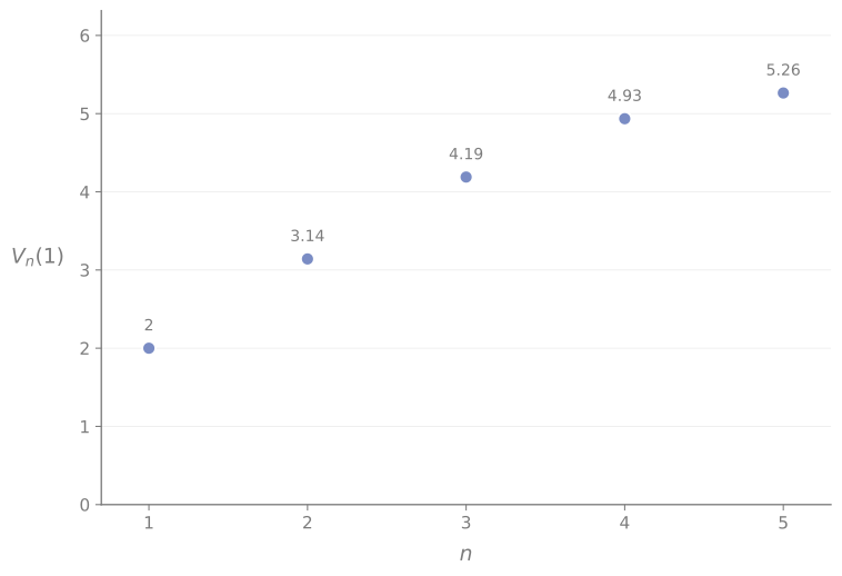
… until we reach $n = 5$. After that, the volume decreases. And not only does it decrease, it decreases superexponentially, faster than any exponential function!

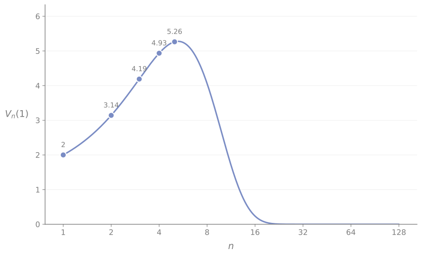
This looks like a very thrilling rollercoaster ride. Not only is the volume asymptotically going to $0$, but beyond a very reasonable $n$ value it is practically zero as well!

For $n=16$ we have

\[V_{16}(1) = \frac{\pi^8}{8!} \approx 0.235,\]

and for $n = 32$ we have

\[V_{32}(1) = \frac{\pi^{16}}{16!} \approx 4.30307 \times 10^{-6} = 0.0000043.\]

For most applications, that is practically zero.

What about a larger ball?

We can try to beat this process by looking at a slightly larger ball, since we would also scale the volume by $R^{n}$. Instead of $R=1$, let’s take $R = 2$ or $R=3$: that should give us a $2^{n}$ and $3^{n}$ scale factor, respectively.

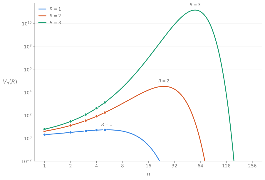
It does not help. There is no escaping the rollercoaster that is the volume of the $n$-ball.

Where is the volume of the $n$-ball?

Consider a very thin shell of the unit $n$-ball, obtained by drawing the $n$-ball with unit radius $R = 1$ and then putting a slightly smaller $n$-ball of radius $0.98R$. What is the ratio of the volume of the inner ball to the outer ball?

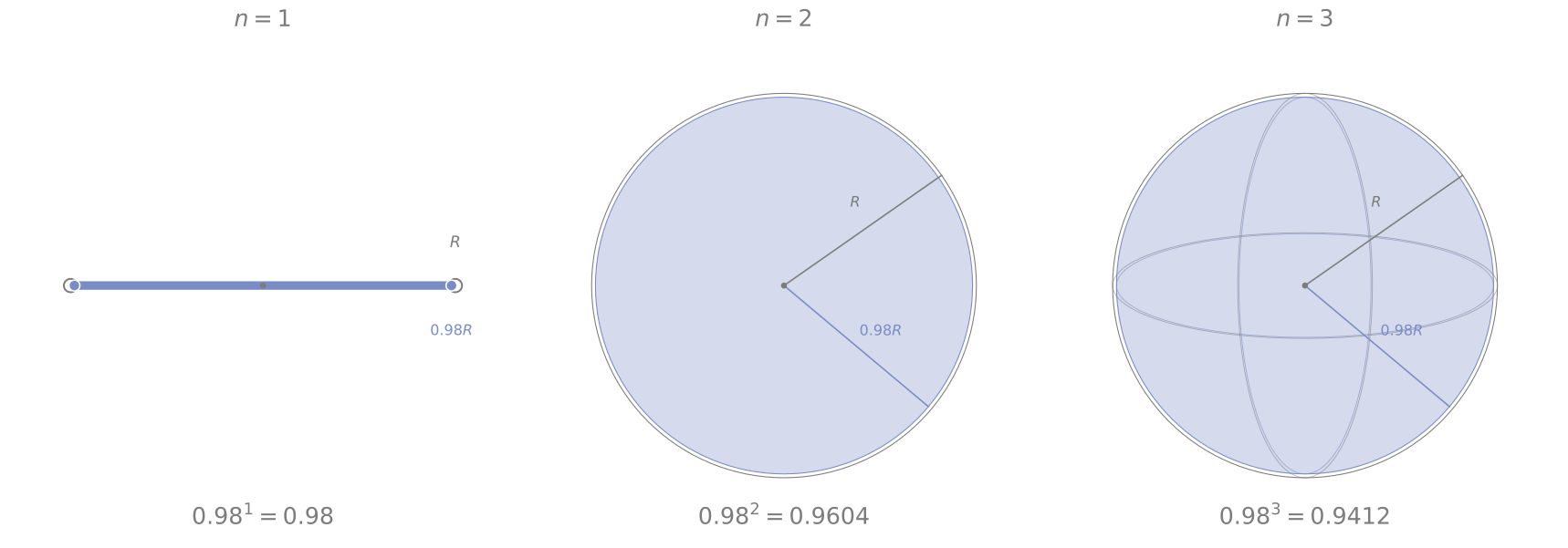
In the figure above, you can barely see the gap between the inner and the outer $n$-balls.

• For $n = 1$, we have

\[\frac{V_{1}(0.98R)}{V_{1}(R)} = \frac{2\cdot 0.98R}{2\cdot R} = 0.98.\]

• For $n = 2$, we have

\[\frac{V_{2}(0.98R)}{V_{2}(R)} = \frac{\pi(0.98R)^2}{\pi R^2} = (0.98)^2 = 0.9604.\]

• For $n = 3$, we have

\[\frac{V_{3}(0.98R)}{V_{3}(R)} = \frac{\frac{4\pi}{3}(0.98R)^3}{\frac{4\pi}{3} R^3} = (0.98)^3 \approx 0.9412.\]

… you get the picture. We start off pretty strong, and visually we can see that most of the volume of the $n$-ball is inside the volume of the smaller $n$-ball.

However, by $n=128$ the ratio is now

\[\frac{V_{128}(0.98R)}{V_{128}(R)} \approx 0.0753.\]

For a $128$-ball, approximately $92.47\%$ of the outer ball’s volume is concentrated in the thin shell!

We can express the specific ratio for some $n$ and $R$ with

\[\begin{align} 1 - \frac{V_{n}(0.98R)}{V_{n}(R)} &= 1 - \frac{C_{n}(0.98R)^{n}}{C_{n}R^n} \\ &= 1 - (0.98)^{n}. \end{align}\]

As $n \rightarrow \infty$, we see that the ratio becomes $1$. There is basically no volume unless you are near the boundary.

Sampling from the unit $n$-ball

We end this one with sampling points in the unit $n$-ball. In my case, it was quite peculiar when I had to deal with it recently.

How do you sample from the $n$-ball of radius $R$? Suppose you have access to the uniform distribution and the normal distribution.

One idea is rejection sampling. It’s very fast and intuitive, let’s look at the 2D case.

1. We sample $x$ and $y$ such that $x,y \sim \mathcal{U}[-1, 1]$ are from the uniform distribution.
2. We calculate $r = \sqrt{x^2 + y^2}$.
3. If $r \leq R$ we keep the sample (it’s in the disk), otherwise we reject it.

Here’s how it looks for 1000 candidate $(x, y)$ pairs in step (1).

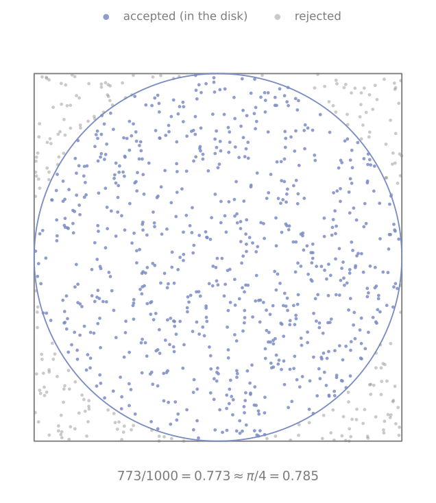
Empirically, $773 / 1000 = 0.773$ were in the disk. On paper, we expect around

\[\frac{\pi\cdot1^2}{2 \times 2} = \frac{\pi}{4} \approx 0.785\]

of sampled points to be valid samples, or

\[1000\cdot\frac{1}{0.785} \approx 1273\]

candidates to successfully sample 1000 points inside the unit disk. As you might expect this doesn’t scale to higher dimensions very well.

For $n=20$ we have

\[\frac{V_{20}(1)}{2^{20}} = \frac{\pi^{10} / 10!}{1048576} \approx 2.46 \times 10^{-8},\]

or approximately

\[1000 \cdot \frac{1}{2.46 \times 10^{-8}} \approx 4 \times 10^{10},\]

or $40000000000$ candidate points just to perhaps sample 1000 points inside the unit $20$-ball. Muller states that it would take

Rejection sampling is basically impossible for higher dimensions, due to its inefficiency.

The Gaussian trick

I’m not sure who the entire process is attributed to, although the normalized Gaussian idea appears to be from (Muller, 1959).

The trick works in three steps.

1. We start by sampling $\mathbf{g} \sim \mathcal{N}(0, I_{n})$, the $n$-dimensional Gaussian distribution. We then normalize it as $\mathbf{v} = \frac{\mathbf{g}}{\lVert \mathbf{g} \rVert}$.

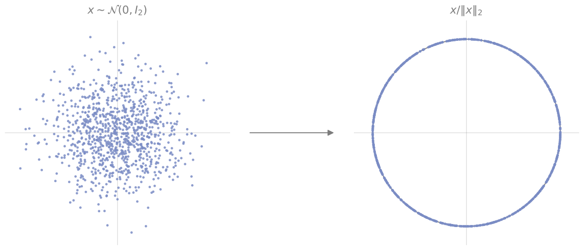
Now, we have to disperse the points on the $n$-sphere with the appropriate radius distribution of the $n$-ball.

2. We sample $u \sim \mathcal{U}[0, 1]$ and let $r = u^{1/n}$.

The product $r \cdot \mathbf{v}$ already gives us a random uniform sample from the unit $n$-ball.

3. Scale it by multiplying with $R$ to randomly sample from the $n$-ball with radius $R$ instead.

After all three steps, the product $R\cdot r \cdot \mathbf{v}$ gives us a uniformly sampled random variable in the $n$-ball with radius $R$, quite efficiently and without any rejection sampling.

Closing remarks

There are many more properties about the $n$-ball that I want to talk about, and this is only scratching the surface. We saw a couple major properties in this post.

• The closed-form volume formula can be derived from the cross-section integral, as we showed in the first section.

• The volume of the $n$-ball is a rollercoaster that briefly rises before plummeting to its doom (zero).

• As $n$ increases, the volume increasingly concentrates near the boundary of the $n$-ball.

• It’s slightly difficult to sample from at first glance, but efficient with some tricks.

Next time, I’ll talk about the surface of the $n$-ball and an alternative formulation for the volume.

References

- Muller, M. E. (1959). A note on a method for generating points uniformly on n-dimensional spheres. Commun. ACM, 2(4), 19–20. https://doi.org/10.1145/377939.377946