The surface of the n-ball

This is the third entry in the high-dimensional space blog series.

Let’s talk about another simple way of calculating the volume of the $n$-ball, with a method that on paper seems more intuitive than the cross-section approach.

I had planned this one to have less math than the previous post, but it turned out to require even more! It’s nice that the “mathy” blocks can be toggled on/off with the “Why?” blocks.

The onion method

Recall that in the volume of the 4-ball, we showed that the 2D disk can be thought of as a vertical stack of horizontal disks, which were actually $1$-balls of varying radii:

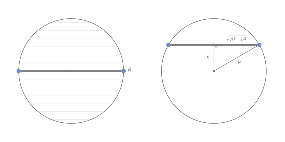
If we’re going to be slicing up the unit ball, there is a much more intuitive way of doing so: radially outwards, like an onion.

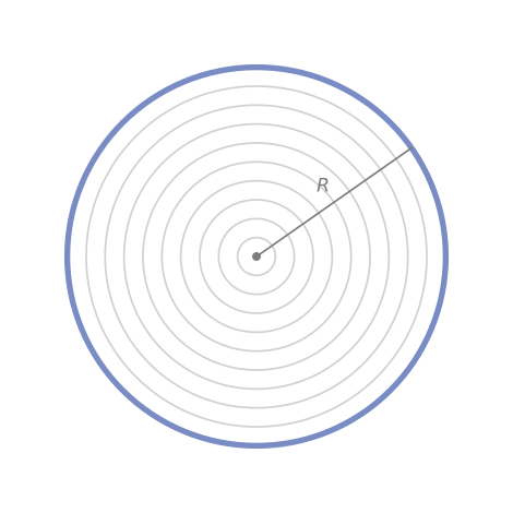
Inside a disk of radius $R$, each one of these circles has a circumference of $2\pi r$ with varying $r \in [0, R]$. The integral for adding all of these circle circumferences gives us the volume:

\[V_{2}(R) = \int_{0}^{R} 2\pi r\,dr = \pi R^{2}.\]

That was pretty easy, wasn’t it?

This also works in the three-dimensional case as well. We know that the surface of the ball of radius $R$ has a surface area of $4\pi R^{2}$, and the $3$-ball can be thought of as a similar 3D onion with infinite layers.

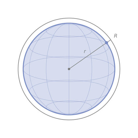
Again, we find that the integral here gives us the volume of the $3$-ball.

\[V_{3}(R) = \int_{0}^{R} 4\pi r^2 \,dr = \frac{4}{3}\pi R^3.\]

The n-dimensional case

So why didn’t we use this for volume of the $n$-ball, as it looks easier to calculate? It’s because we didn’t know the surface area of the $n$-ball, of course!

We actually go the other way around: the surface area $S_{n-1}(R)$ for the $n$-ball is the volume of the $(n-1)$-sphere, and is equal to the rate of change of the volume of the $n$-ball with respect to the radius:

\[\begin{align} S_{n-1}(R) &= \frac{d}{dR}V_{n}(R) \\ &= \boxed{\frac{2\pi^{n/2}}{\Gamma(n/2)}R^{n-1}}. \label{eq:eq1} \tag{1} \end{align}\]

And by our onion construction, we can express the volume of the $n$-ball using the volume of the $(n-1)$-sphere as

\[\boxed{V_{n}(R) = \int_{0}^{R} S_{n-1}(r)\,dr}. \label{eq:eq2} \tag{2}\]

Why?

Suppose we are looking at the difference between $V_{n}(R)$ and $V_{n}(R + h)$ for some $h > 0$. Intuitively, this is the volume of the shell between two nested $n$-balls, and as $h \to 0$ this approximates the boundary of the ball of radius $R$, which is the sphere of radius $R$ multiplied by a height of $h$.

\[\begin{align} V_n(R+h) - V_n(R) &\approx S_{n-1}(R)\cdot h \\ \quad\Longrightarrow\quad S_{n-1}(R) &= \lim_{h\to 0}\frac{V_n(R+h) - V_n(R)}{h} = V_n'(R). \end{align}\]

Therefore we have

\[\begin{align} S_{n-1}(R) := V'_{n}(R) &= \frac{d}{dR} \left[\frac{\pi^{n/2}}{\Gamma(n/2 + 1)}R^{n}\right] \\ &= \frac{\pi^{n/2}}{\Gamma(n/2 + 1)}\cdot\frac{d}{dR}[R^n] \\ &= \frac{\pi^{n/2}}{\Gamma(n/2 + 1)}\cdot n \cdot R^{n-1} \\ &= \frac{\pi^{n/2}}{\frac{n}{2}\Gamma(n/2)}\cdot n \cdot R^{n-1} \\ &= \frac{2\pi^{n/2}}{\Gamma(n/2)}R^{n-1}. \end{align}\]

which recovers \eqref{eq:eq1}. It then follows from $S_{n-1}(R) = \frac{d}{dR}V_{n}(R)$ that

\[\int_{0}^{R} S_{n-1}(r)\,dr = V_{n}(R) - V_{n}(0) = V_{n}(R),\]

which gives us \eqref{eq:eq2}.

Does the onion method always work?

In the volume post, there was one nice property that we didn’t touch upon: Fubini’s theorem and the cross-section idea work not just for Euclidean distance, but for other norms as well.

An $\ell_{p}$ norm for a vector $\mathbf{u} \in \mathbb{R}^n$ is a measure for the length of a vector $\mathbf{u}$, defined as:

\[\ell_{p}(\mathbf{u}) = \lVert \mathbf{u} \rVert_{p} = \left(\lvert u_{1}\rvert^{p} + \lvert u_{2}\rvert^p + \cdots + \lvert u_{n}\rvert^p\right) ^{1/p}.\]

For $p=2$, this is our good old Euclidean distance, for example for $\mathbf{u} \in \mathbb{R}^3$ with $\mathbf{u} = (x, y, z)$:

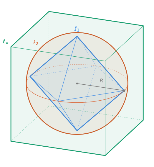
\[\ell_{2}(\mathbf{u}) = \lVert \mathbf{u} \rVert_{2} = \sqrt{x^2 + y^2 + z^2}.\]

The shapes below are all $3$-balls, just with different norms.

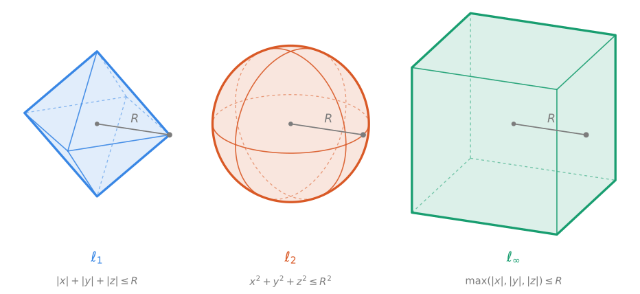
The green ball (cube) uses the max norm. The max-norm is the resulting norm we have as $p \to \infty$. It is defined as

\[\ell_{\infty}(\mathbf{u}) = \lVert \mathbf{u} \rVert_{\infty} = \max\left\{|u_{1}|, |u_{2}|, \cdots ,|u_{n}| \right\}.\]

What’s also cool is that they all encapsulate each other with increasing $p$:

We’re going to talk about norms and distances in greater detail in a later post.

So why talk about the norm now?

Our onion approach is a special case of the $\ell_2$ (Euclidean) norm. Interestingly enough, it also holds for the $\ell_{\infty}$ norm as well.

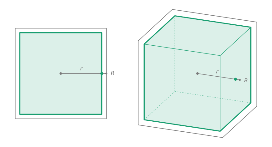
• With $\ell_{\infty}$, the “$1$-sphere” of radius $r$ gives us a square of $4$ edges of length $2r$. Integrating this gives us

\[V_{2}(R) = \int_{0}^{R} 4\cdot2r\,dr = 4R^2,\]

which is the volume of the “$2$-ball” here, the square of edge length $2R$.

• In 3D this again holds: a max norm $2$-sphere of radius $r$ has $6$ faces of surface area $2r \times 2r = 4r^2$, and integrating gives us

\[V_{3}(R) = \int_{0}^{R} 6 \cdot 4r^{2}\,dr = 8 R^3,\]

which is again the volume of the $3$-ball with max norm, in other words, a cube with edge length $2R$ with volume $(2R)^3 = 8R^3$.

---

For other norms though, we have the issue of slantedness. It’s most intuitively observed in the figure below for the disk with various $\ell_{p}$ norms.

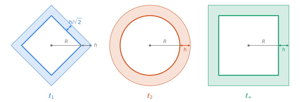
In our argument above we said that for sufficiently small $h > 0$ the difference between the volumes of the $n$-ball of radius $(R+h)$ and $R$ can be approximated by $S_{n-1}(R) \cdot h$.

Uniquely for $\ell_{2}$ and $\ell_{\infty}$, we see that increasing the radius $R$ by some $h$ directly pushes the outer shell away by $h$, whereas there is a slant factor for all other $\ell_{p}$ norms (for example, $\ell_{1}$ has $\frac{h}{\sqrt{2}}$ instead). That means we can’t use the $S_{n-1}(R) \cdot h$ volume approximation for the other norms.

The rollercoaster of the volume of the $(n-1)$-sphere

Given that Eq. \eqref{eq:eq1} looks awfully similar to the $n$-ball volume formula, we might expect this next property: the volume $S_{n-1}(R)$ of the $(n-1)$-sphere with radius $R$ also increases for a bit before superexponentially plummeting to zero.

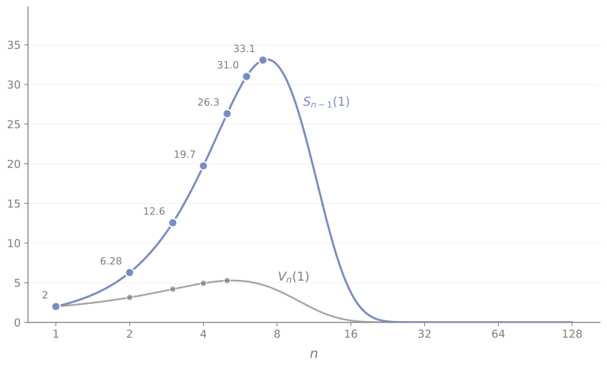
Note that the unit $n$-ball volume peaks at $n=5$, while the unit $(n-1)$-sphere volume peaks at $n=7$ (i.e., with the $6$-sphere). Similar to the $n$-ball volume, increasing the radius only prolongs the inevitable.

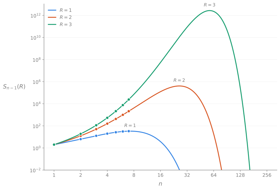
It’s still quite surprising, but not as much as before given that it’s basically the same argument as the $n$-ball.

The equator phenomenon

The principle holds here for the surface as well, but I want to look at this topic through the perspective of the volume of the $n$-ball. I think the general idea and a similar bound come from (Ball, 1997).

Consider the unit $n$-ball centered in the origin. Pick any direction $\mathbf{u}$, and consider the normal hyperplane to that direction passing through the origin: that is the equator. If we consider a band of width $2/\sqrt{n}$ around this equator, what is the fraction of the volume of the $n$-ball within this band?

Here’s how it looks for 2D and 3D:

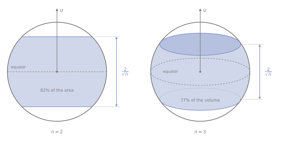
The band stands out relatively wide and as we increase the dimension, both the width of the band, as well as the ratio of the volume of the equator band to the unit ball start decreasing. But they don’t decrease in the same manner.

---

Let’s try to visualize what happens when we increase the dimension, such as $n = 400$. Even though we can’t directly visualize a $400$-ball, we can show its 2D projection while trying to accurately represent the approximate density of the ball at each point while moving along the direction of $\mathbf{u}$:

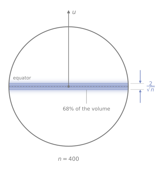
That looks quite unbelievable! It is fascinating how this thin equator band contains $\approx 68.3\%$ of the total volume of the $n$-ball, given that we can repeat it along any random direction and still its corresponding equator band will have the same percentage of the total volume. They all look like they share the “center” section, but let’s also not forget that the volume of the $n$-ball is also concentrated near the surface of the sphere, the center has basically no volume.

What is more interesting is that as we further increase $n$, the band grows thinner and thinner, while the volume ratio of the equator band to the unit ball stays $\approx 68.3\%$.

Why?

Let’s use our cross-section machinery from the volume post: consider the unit ball (and the equator band) as a stack of $(n-1)$-dimensional balls along the direction vector $\mathbf{u}$, with varying radii $r_t = \sqrt{1 - t^2}$.

The practical result is that at each point $t$ along the direction of $\mathbf{u}$, the density of the ball scales with $V_{n-1}(r_t)$. To see this, we use $V_{n}(R) = C_{n}R^{n}$:

\[\begin{align} V_{n-1}(\sqrt{1-t^2}) &= C_{n-1} \left( \sqrt{1-t^2} \right)^{n-1} \\ &= C_{n-1} (1 - t^2)^{(n-1)/2}. \end{align}\]

Normalizing this by the unit ball volume $V_{n}(1)$ and integrating along the entire ball gives us $1$ per the cross-section formula from the previous post.

\[\begin{align} \int_{-1}^{1}\frac{V_{n-1}(\sqrt{1-t^2})}{V_{n}(1)}\,dt &= \int_{-1}^{1}\frac{C_{n-1} (1-t^2)^{(n-1)/2}\,dt}{C_{n}\cdot 1^{n}} \\ &= \int_{-1}^{1}\underbrace{\frac{C_{n-1}}{C_{n}}\cdot(1-t^2)^{(n-1)/2}}_{p(t)}\,dt. \end{align}\]

Since $\frac{C_{n-1}}{C_n}$ is constant, this shows that the probability density function $p(t)$ scales with

\[(1-t^2)^{(n-1)/2}.\]

Why specifically 0.683?

We have to look at the volume of the equator band compared to the volume of the unit $n$-ball.

The ratio of the two volumes in $n$ dimensions, $\rho_{n}$, is equal to

\[\begin{align} \rho_{n} &= \frac{\int_{-1/\sqrt{n}}^{1/\sqrt{n}}V_{n-1}(r_{t})\,dt}{V_{n}(1)} \\ &= \frac{\int_{-1/\sqrt{n}}^{1/\sqrt{n}}\frac{\pi^{(n-1)/2}}{\Gamma((n-1)/2 + 1)}\left(\sqrt{1-t^2}\right)^{n-1}\,dt}{\frac{\pi^{n/2}}{\Gamma(n/2 + 1)}} \\ &= \frac{\frac{\pi^{(n-1)/2}}{\Gamma((n-1)/2 + 1)}\int_{-1/\sqrt{n}}^{1/\sqrt{n}}\left(1-t^2\right)^{(n-1)/2}\,dt}{\frac{\pi^{n/2}}{\Gamma(n/2 + 1)}} \\ &= \frac{\pi^{(n-1)/2}}{\pi^{n/2}} \cdot \frac{\Gamma(n/2 + 1)}{\Gamma((n-1)/2 + 1)} \cdot 2 \int_{0}^{1/\sqrt{n}}(1-t^2)^{(n-1)/2}\,dt \\ &= \frac{2}{\sqrt{\pi}}\cdot \frac{\Gamma(n/2 + 1)}{\Gamma((n-1)/2 + 1)} \cdot \int_{0}^{1/\sqrt{n}}(1-t^2)^{(n-1)/2}\,dt. \end{align}\]

This two-part form doesn’t simplify any further, but taking the limit $n \to \infty$ allows us to progress with the parts individually. I was stuck on this part for some time on these limits, and Claude helped with the following parts:

First, taking the limit properly for these two needs the following adjustment:

\[\rho_n = \sqrt{\frac{2}{\pi}}\cdot \underbrace{\frac{\Gamma(n/2+1)}{\sqrt{n/2}\,\Gamma((n-1)/2+1)}}_{A_n}\cdot \underbrace{\sqrt{n}\int_{0}^{1/\sqrt{n}}(1-t^2)^{(n-1)/2}\,dt}_{B_n}.\]

Now we look at them individually.

• For $A_{n}$, we have the ratio of Gamma functions resulting in

\[\lim_{n\to\infty}A_{n} = 1.\]

This is shown in the appendix.

• For $B_{n}$, we first substitute $t = u / \sqrt{n}$ to get

\[B_{n} = \sqrt{n}\int_{0}^{1/\sqrt{n}}(1-t^2)^{(n-1)/2}\,dt = \int_{0}^{1}\left(1-\frac{u^2}{n}\right)^{(n-1)/2}\,du.\]

We then look at $\lim_{n\to\infty}B_{n}$. The integrand $(1-u^2/n)^{(n-1)/2}$ is bounded and converges for every $u$ on $[0, 1]$, so by the dominated convergence theorem we can take the limit inside the integral and apply the identity $\lim_{n\to\infty}(1 + a/n)^{n} = e^{a}$:

\[\begin{align} \lim_{n\to\infty}B_{n} &= \lim_{n\to\infty}\int_{0}^{1}\left(1-\frac{u^2}{n}\right)^{(n-1)/2}\,du \\ &=\int_{0}^{1}\lim_{n\to\infty}\left[\left(1-\frac{u^2}{n}\right)^{n}\right]^{1/2}\cdot \left(1-\frac{u^2}{n}\right)^{-1/2}\,du \\ &= \int_{0}^{1}\left(e^{-u^2}\right)^{1/2}\cdot1^{-1/2}\,du \\ &= \int_{0}^{1}e^{-u^2/2}\,du. \end{align}\]

---

So, the product as $n\to\infty$ is then the product of these limits:

\[\begin{align} \lim_{n\to\infty}\rho_{n} &= \sqrt{\frac{2}{\pi}} \cdot 1 \cdot \int_{0}^{1}e^{-u^2/2}\,du \\ &= \sqrt{\frac{2}{\pi}}\int_{0}^{1}e^{-u^2/2}\,du. \end{align}\]

Finally, we substitute $u = \sqrt{2}\,s$ to transform the integral into the form of the error function:

\[\begin{align} \lim_{n\to\infty}\rho_{n} &= \sqrt{\frac{2}{\pi}}\cdot \sqrt{2} \cdot \int_{0}^{1/\sqrt{2}}e^{-s^2}\,ds \\ &= \mathrm{erf}(1/\sqrt{2}) \\ &\approx 0.683. \tag*{$\Box$} \end{align}\]

We used $\mathrm{erf}(x) = \frac{2}{\sqrt{\pi}}\int_{0}^{x}e^{-s^2}\,ds$ in the last part above.

---

Another intuitive way to visualize this is to directly look at the marginal distribution of the points of the $n$-ball onto the 1D line of the direction vector $\mathbf{u}$:

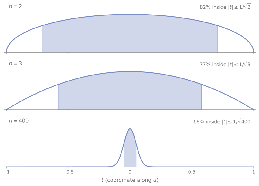
The marginal distributions above show how the distribution of points along a random direction changes as $n$ increases. For high dimensions, $68.3\%$ of points lie within the band of $2/\sqrt{n}$ width. This is slightly intuitive when we consider that most individual coordinates for randomly sampled points on the sphere should have magnitude close to $1/\sqrt{n}$, which is one of the core ideas for a following post on angles in high-dimensional space.

A practical note on “Why the surface?”

One thing that frequently pops up in machine learning is to normalize high-dimensional samples from a dataset for reasons like measuring cosine similarity or retrieving samples. Given a sample $\mathbf{x} \in \mathbf{X} \subset \mathbb{R}^d$, L2-normalizing the sample $\mathbf{x} \leftarrow \frac{\mathbf{x}}{ \lVert \mathbf{x} \rVert}$ puts it on the surface of the $d$-dimensional unit ball, i.e., the $(d-1)$-dimensional unit sphere.

Representation spaces are commonly $512$, $768$ or $1024$-dimensional for stuff like word embeddings (see a previous post for an example) and vision-language embeddings (e.g., CLIP, SigLIP), where both the volume and surface area are practically in the funky high-dimensional regime, looking at the volume scaling graph.

Hopefully, now we have a bit more insight towards the fact that this $(d-1)$-sphere does not have our 2D or 3D expectations in appearance, distribution, or concentration of volume.

Appendix

The limit of the Gamma ratio

Recall that we’re concerned with the limit

\[\begin{align} \lim_{n\to\infty}A_{n} &= \lim_{n\to\infty}\frac{\Gamma(n/2 + 1)}{\Gamma((n-1)/2 + 1)\sqrt{n/2}}. \end{align}\]

Let $g(x) = \frac{\Gamma(x+1)}{\Gamma(x + \frac{1}{2})}$. We’re going to need $g(n/2)$. We have the very useful property of

\[g(x)g(x-\frac{1}{2}) = \frac{\Gamma(x+1)}{\Gamma(x + \frac{1}{2})} \cdot \frac{\Gamma(x+\frac{1}{2})}{\Gamma(x)} = \frac{\Gamma(x+1)}{\Gamma(x)} = x,\]

using $\Gamma(z+1)=z\,\Gamma(z)$.

Similarly, we see that

\[g(x)g(x+\frac{1}{2}) = x + \frac{1}{2}.\]

The function $g(x)$ is monotonically increasing, since $\log\Gamma(x)$ is convex (a commonly known property). Thus we have

\[g(x - \frac{1}{2}) \leq g(x) \leq g(x + \frac{1}{2}).\]

Multiply everything by $g(x) > 0$:

\[g(x)g(x - \frac{1}{2}) \leq g^2(x) \leq g(x)g(x + \frac{1}{2}).\]

Using the identities we just proved:

\[x \leq g^2(x) \leq x + \frac{1}{2},\]

then take the square root:

\[\sqrt{x} \leq g(x) \leq \sqrt{x + \frac{1}{2}}.\]

Divide by $\sqrt{x}$ to get

\[1 \leq \frac{g(x)}{\sqrt{x}} \leq \sqrt{1 + \frac{1}{2x}},\]

and finally substitute $x = n/2$ to recover $A_{n}$:

\[1 \leq \frac{g(n/2)}{\sqrt{n/2}} = \frac{\Gamma(n/2 + 1)}{\Gamma((n-1)/2 + 1)\sqrt{n/2}} = A_{n} \leq \sqrt{1 + \frac{1}{n}}.\]

All that’s left is to look at the limit as $n\to\infty$. We have

\[\lim_{n\to\infty} 1 = \lim_{n\to\infty}\sqrt{1 + \frac{1}{n}} = 1.\]

Therefore, by the squeeze theorem we have

\[\lim_{n\to\infty}A_{n} = 1. \tag*{$\Box$}\]