The n-dimensional Gaussian

This is the fourth entry in the high-dimensional space blog series.

The normal distribution is everywhere in machine learning. Off of the top of my head, we use it for

• Modeling measurement error and uncertainty (Gauss’s starting point)
• A popular choice for the prior of a latent distribution
• Sampling noise for methods such as autoencoders and GANs
• As a target distribution for learned representations, most recently seen in (Balestriero & LeCun, 2025).

among many others. Our goal today is to look at the multivariate ($n$-dimensional) normal distribution in high-dimensional space.

Recalling the Gaussian

The normal (or Gaussian) distribution $\mathcal{N}(x; \mu, \sigma^2)$ for $x \in \mathbb{R}$ is defined with the following probability density function in the single variable case:

\[\mathcal{N}(x;\mu, \sigma^2) = \frac{1}{\sqrt{2\pi\sigma^2}}\exp\left\{-\frac{(x - \mu)^2}{2\sigma^2}\right\}.\]

We usually drop the $x$ part and write $\mathcal{N}(\mu, \sigma^2)$.

Visually, we know it more commonly as the “bell curve”:

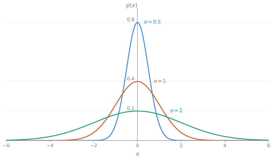
Note that while the probability decreases exponentially with distance from the mean, the possible values for $x$ technically range from $-\infty$ to $\infty$.

---

The normal distribution also has the corresponding cumulative distribution function (CDF), which is obtained by integrating the pdf from $-\infty$ to a target $x$:

\[\Phi(x) = \frac{1}{\sqrt{2\pi}}\int_{-\infty}^{x}e^{-t^2/2}\,dt.\]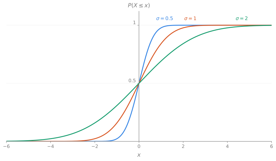

As $\sigma$ increases the distribution becomes flatter, and as a result the CDF converges to $1$ more slowly. In the opposite direction, as $\sigma\to 0$ the peak of the PDF gets sharper until it becomes an infinitely tall spike on $x=\mu$ with total mass 1 (i.e., a Dirac delta function), which produces a step function as the CDF.

Given the historical context that we’ll uncover later in the article, from this point on I’ll refer to the distribution as the Gaussian.

Two core properties of the Gaussian

We briefly go over the two most “obvious” but crucial properties of the distribution.

• The mean of the Gaussian is $\mathbb{E}[X] = \mu$.

• The variance of the Gaussian is $\mathbb{V}[X] = \sigma^2$.

Why?

Let’s start with the mean. We have

\[\mathbb{E}[X] = \int_{-\infty}^{\infty} x\,p(x)\,dx = \frac{1}{\sqrt{2\pi \sigma^2}}\int_{-\infty}^{\infty} x\,e^{-(x-\mu)^2/2\sigma^2}\,dx.\]

Let $u = (x - \mu)/\sigma$, with $du = (1/\sigma)\,dx$. Then

\[\begin{align} \mathbb{E}[X] &= \frac{1}{\sqrt{2\pi\sigma^2}}\int_{-\infty}^{\infty} (\mu + \sigma\,u) \cdot e^{-u^2/2}\cdot \sigma\,du \\ &= \frac{1}{\sqrt{2\pi}} \int_{-\infty}^{\infty} (\mu + \sigma\,u) \cdot e^{-u^2/2}\cdot\,du \\ &= \frac{\mu}{\sqrt{2\pi}} \int_{-\infty}^{\infty}e^{-u^2/2}\,du + \frac{\sigma}{\sqrt{2\pi}}\int_{-\infty}^{\infty}u\,e^{-u^2/2}\,du \\ &= \frac{\mu}{\sqrt{2\pi}}\cdot\sqrt{2\pi} + \frac{\sigma}{\sqrt{2\pi}}\left[-e^{-u^2/2}\right]_{-\infty}^{\infty} \\ &= \mu + (0 - 0) \\ &= \mu. \end{align}\]

The intermediate $\int_{-\infty}^{\infty} e^{-u^2/2}\,du = \sqrt{2\pi}$ can be verified by the simple substitution $v^2 = u^2/2, 2v\,dv = u\,du$, followed by the classical polar coordinates trick for $\int_{-\infty}^{\infty}e^{-v^2}\,dv = \sqrt{\pi}$. We showed this in an earlier post.

---

For the variance, let’s use

\[\mathbb{V}[X] = \mathbb{E}[(X - \mathbb{E}[X])^2] = \mathbb{E}[(X - \mu)^2],\]

since we just showed at $\mathbb{E}[X] = \mu$ above. With LOTUS, we have

\[\begin{align} \mathbb{V}[X] = \mathbb{E}[(X - \mu)^2] & = \frac{1}{\sqrt{2\pi\sigma^2}}\int_{-\infty}^{\infty}(x-\mu)^2 e^{-(x-\mu)^2/2\sigma^2}\,dx \\ \end{align}\]

We substitute $u = x-\mu$ to get

\[\begin{align} \mathbb{V}[X] = \frac{1}{\sqrt{2\pi\sigma^2}}\int_{-\infty}^{\infty}u^2\,e^{-u^2/2\sigma^2}\,du. \\ \end{align}\]

The integrand calls for IBP here, with $a = u$ and $db = u\,e^{-u^2/2\sigma^2}\,du$. With these we have

\[\begin{align} da &= du, \\ b &= \int u\,e^{-u^2/2\sigma^2}\,du = -\sigma^2\,e^{-u^2/2\sigma^2}, \end{align}\]

and so by IBP we have

\[\begin{align} \mathbb{V}[X] &= \frac{1}{\sqrt{2\pi\sigma^2}}\left[a\,b \Big|_{-\infty}^{\infty} - \int_{-\infty}^{\infty}b\,da\right] \\ &= \frac{1}{\sqrt{2\pi\sigma^2}} \left[ u\cdot -\sigma^2 e^{-u^2/2\sigma^2}\Big|_{-\infty}^{\infty} - \int_{-\infty}^{\infty}(-\sigma^2)e^{-u^2/2\sigma^2}\,du\right] \\ &= \frac{1}{\sqrt{2\pi\sigma^2}} \left[0 + \sigma^2 \int_{-\infty}^{\infty} e^{-u^2/2\sigma^2}\,du\right] \\ &= \frac{1}{\sqrt{2\pi\sigma^2}} \cdot \sigma^2 \cdot \sqrt{2\pi\sigma^2} \\ &= \sigma^2. \end{align}\]

Here, we made use of two things. The term $u\,e^{-u^2/2\sigma^2}$ goes to zero for both $-\infty$ and $\infty$ because the exponential term dominates. And again, we face an integral of the form $I_{\alpha}= \int_{-\infty}^{\infty}e^{-\alpha u^2}\,du$, with $\alpha = 1/2\sigma^2$, which has the general result of $I_{\alpha} = \sqrt{\pi / \alpha}$ for $\alpha > 0$.

While these are well known, deriving them from scratch feels somewhat reassuring.

Where does the Gaussian come from?

As its alternative name suggests, the Gaussian distribution is attributed to Gauss, although de Moivre derived the curve as an approximation to binomial probabilities for many trials (de Moivre, 1738).

We’ll go with Gauss’s starting point of modeling measurement error.

The setup

Suppose we’re taking many measurements $x_1, x_2, \cdots, x_n$ of some unknown quantity $\mu$, and each measurement sample is independent and identically distributed. As we accrue more measurements, the values $x_i$ seem to form a bell curve, but we don’t know the underlying function that explains the curve. Let’s name the measurement density $p(x)$, and the error density function $\varphi(x)$, with $\varphi(x-\mu) = p(x)$.

We have an initial guiding principle to follow: the resulting distribution of $p(x)$ is smooth, symmetrical, and has a single peak which is its mean $\mu$. Likewise, $\varphi(e)$ shares the same properties, and its peak is specifically $0$.

\[\mathbb{E}[X - \mu] = \mathbb{E}[e] = 0.\]

However, note that this doesn’t uniquely determine the Gaussian. In fact, look how similar a Gaussian and a logistic distribution look:

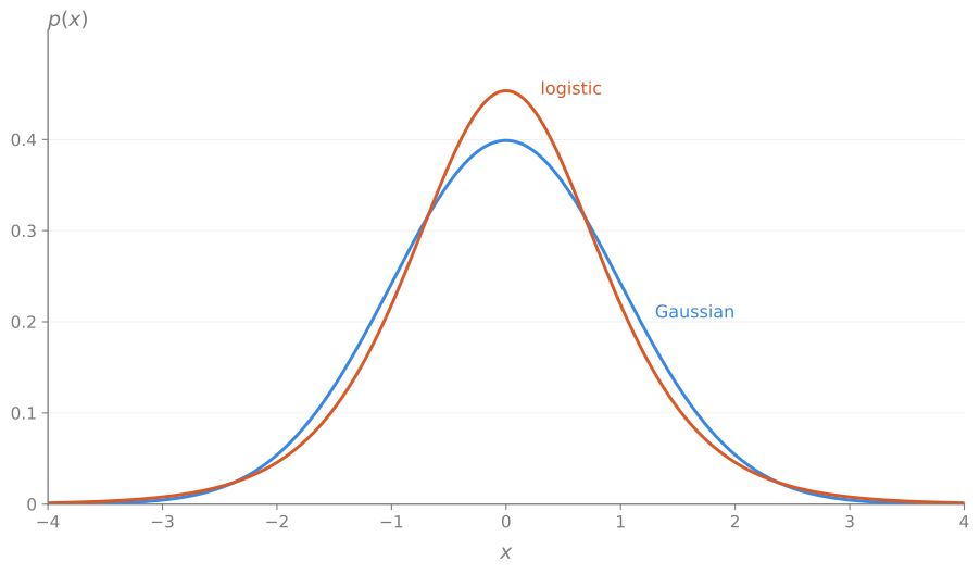
They are both smooth and symmetric, and aside from the logistic function’s heavier tail, there is little discernible detail between them visually. The Gaussian distribution arises from the following postulate.

The rest of the derivation goes into a bit of detail, so I’ll wrap it up in a dropdown block.

Deriving the Gaussian distribution

By the postulate above, the maximum likelihood estimate (MLE) is

\[\arg\max_{\mu}\prod_{i=1}^{n} \varphi(x_{i} - \mu) = \bar{x},\]

for every $n$ and every dataset $\mathcal{D}$.

With the MLE our instinct is to convert it to log-likelihood, and set its derivative to zero.

\[\begin{align} \frac{d}{d\mu}\left[\sum_{i=1}^{n}\log\varphi(x_i-\mu)\right] &= -\sum_{i=1}^{n}\frac{\varphi'(x_i - \mu)}{\varphi(x_i - \mu)} = 0. \end{align}\]

Let $g(t) = \varphi’(t)/\varphi(t)$, so that we have

\[\sum_{i=1}^{n}g(x_{i} - \mu) = 0.\]

Recall from the postulate that the maximum likelihood solution is $\mu = \bar{x}$, i.e.,

\[\sum_{i=1}^{n}g(x_i - \bar{x}) = 0.\]

Let’s call the $r_i = x_i - \bar{x}$ the error residuals, which are actual quantities we have at our disposal; remember that we don’t know $\mu$, so we don’t have the errors $e_i = x_i - \mu$.

We know that these residuals always sum up to zero:

\[\sum_{i}^{n}r_{i} = \sum_{i}^{n}[x_i - \bar{x}] = \underbrace{(x_1 + \cdots + x_n)}_{n \cdot \bar{x}} - \, n\cdot \bar{x} = 0.\]

And from the postulate we know that their $g(\cdot)$ values also sum up to zero:

\[\sum_{i}^{n}g(x_i - \bar{x}) = \sum_{i}^{n}g(r_i) = 0,\]

for every $n$ and every dataset $\mathcal{D}$. Given this, we can construct some datasets that give more information about the structure of $\varphi$.

---

Case 1

For $\mathcal{D} = \{x_1, x_2\}$ with $x_1 + x_2 = 0$, we have $\bar{x} = 0$ and

\[\sum_{i=1}^{n}g(x_{i}) = g(x_1) + g(x_2) = 0.\]

This means that we have

\[x_1 = -x_2 \qquad \Longrightarrow \qquad g(x_1) = -g(x_2), \tag{1} \label{eq:eq1}\]

which establishes that $g$ is an odd function:

\[g(a) = -g(-a) \qquad \forall a \in \mathbb{R}.\]

---

Case 2

For another $\mathcal{D} = \{x_1, x_2, x_3 \}$ with $x_1 + x_2 = -x_3$, we again have $\bar{x} = 0$ and

\[\sum_{i=1}^{n}g(x_{i}) = g(x_1) + g(x_2) + g(x_3) = 0.\]

Moreover, from \eqref{eq:eq1} we have $g(x_3) = -g(-x_3)$. This gives

\[\begin{align} g(x_1) + g(x_2) &= -g(x_3) \\ &= g(-x_3) \\ &= g(x_1 + x_2). \tag{2} \label{eq:eq2} \end{align}\]

This is Cauchy’s functional equation.

---

The only way to have the smooth, continuous $g$ satisfy both \eqref{eq:eq1} and \eqref{eq:eq2} is if $g(x)$ is a linear function, i.e.,

\[g(x) = \frac{\varphi'(x)}{\varphi(x)} = \alpha\cdot x \qquad \text{for some } \alpha \in \mathbb{R},\]

and from this we derive that $\varphi(x)$ must be in the form of

\[\begin{align} \int \frac{\varphi'(x)}{\varphi(x)}\,dx &= \int \alpha x\,dx \\ \log\varphi(x) &= \frac{\alpha x^2}{2} + c \\ \varphi(x) &= C e^{\alpha x^2 / 2} \qquad \text{for some } C > 0. \end{align}\]

We’ve recovered the general structure of $\varphi(x)$:

\[\boxed{\varphi(x) = Ce^{\alpha x^2/2}}.\]

We now have to find what this $C$ is.

---

Let us recall that $\varphi(x)$ corresponds to the density function of an actual probability distribution. In other words, we need it to integrate to 1:

\[\int_{-\infty}^{\infty} \varphi(x)\,dx = \int_{-\infty}^{\infty}Ce^{\alpha x^2/2}\,dx = 1.\]

This is only possible by having $\alpha < 0$, so let’s use $\tau > 0$ and describe $\varphi$ with $-\tau$ instead:

\[\varphi(x) = C e^{-\tau x^2/2}.\]

Now we have

\[C \int_{-\infty}^{\infty}e^{-(\tau/2)x^2}\,dx = 1.\]

Earlier during our derivation of the variance, we used the identity $\int_{-\infty}^{\infty}e^{-\beta x^2}\,dx = \sqrt{\pi/\beta}$. We can again use it here with $\beta = \tau/2$, which gives $\sqrt{2\pi/\tau}$. Then the normalizing constant $C$ is

\[C \int_{-\infty}^{\infty}e^{(-\tau/2)x^2}\,dx = C \cdot \sqrt{\frac{2\pi}{\tau}} = 1 \qquad \Longrightarrow \qquad C = \sqrt{\frac{\tau}{2\pi}}.\]

Putting it all together, we have

\[\varphi(x) = \sqrt{\frac{\tau}{2\pi}}e^{-\tau x^2/2}.\]

Using $p(x) = \varphi(x - \mu)$, we recover the Gaussian distribution density function $p(x)$ as

\[p(x) = \varphi(x - \mu) = \sqrt{\frac{\tau}{2\pi}}e^{-\tau (x - \mu)^2 /2}.\]

This is a perfectly viable definition of the Gaussian distribution, using $\tau$ as the precision of the distribution. However, the standard formulation is by its variance $\sigma^2$, which we can obtain by the substitution $\tau = 1/\sigma^2$:

\[\boxed{\mathcal{N}(x; \mu, \sigma^2) = \frac{1}{\sqrt{2\pi \sigma^2}} e^{-(x-\mu)^2/2\sigma^2}} \tag*{$\Box$}\]

The advantage of the $\sigma^2$-based parametrization is that we have the nice property of $\mathbb{V}[X] = \sigma^2$.

The multivariate Gaussian

We address the $n$-dimensional Gaussian more commonly as the multivariate normal distribution. It is the extension of the 1D case into multiple dimensions. The general form of the probability density function for the $n$-dimensional Gaussian is

\[\mathcal{N}(\boldsymbol{\mu}, \mathbf{\Sigma}) = \frac{1}{(\sqrt{2\pi})^{n}}\cdot\frac{1}{\sqrt{\det\mathbf{\Sigma}}}\cdot \exp\left\{-\frac{1}{2}(\mathbf{x} - \boldsymbol{\mu})^{\top}\mathbf{\Sigma}^{-1}(\mathbf{x} - \boldsymbol{\mu})\right\},\]

where $\boldsymbol{\mu} \in \mathbb{R}^{n}$ is the mean vector and $\mathbf{\Sigma}$ is a symmetric covariance matrix between the dimensions of the distribution. If we squint at it, it does resemble its univariate form.

The core property to remember is that each dimension in the distribution is itself a Gaussian distribution.

The multivariate Gaussian has two main categories, depending on the structure of its covariance matrix.

Isotropic Gaussians

An isotropic multivariate Gaussian is one where each dimension has the same variance $\sigma^2$, so $\mathbf{\Sigma} = \sigma^2\,I$:

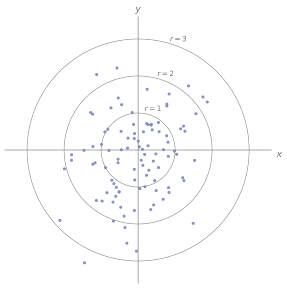
They’re generally nice to work with.

We will later relate the $n$-dimensional unit ball to the $n$-dimensional isotropic Gaussian distribution. This intuitively makes a lot of sense because the unit ball and the isotropic Gaussian centered at the origin share a property called rotational invariance.

Anisotropic Gaussians

A multivariate Gaussian can also be anisotropic, which means the individual dimensions have different variance and can correlate with each other:

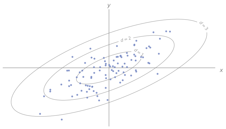
However, note that we can translate and rotate a Gaussian (i.e., choose new bases) and rescale each dimension’s variance to convert it into a standard normal distribution $\mathcal{N}(0, I_n)$. This is a common process known as whitening; all anisotropic Gaussians can be converted to isotropic Gaussians in this way.

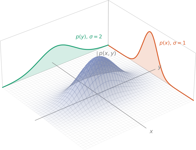
The figure below shows that anisotropic Gaussians are still constructed out of 1D Gaussian distributions:

Scaling the Gaussian to high dimensions

Let’s look at the concentration of density of the Gaussian, as we did for the $n$-dimensional unit ball earlier.

How far away is the typical point?

We have two similar ideas of the “mean” distance of a point. Our random variable of concern is $X \sim \mathcal{N}(\mu, \sigma^2)$.

RMS distance

The first one is the simple root-mean-square (RMS) distance, defined by

\[d_{\mathrm{RMS}} = \sqrt{\mathbb{E}[(X - \mu)^2]}\]

For the univariate Gaussian, we know that

\[\sqrt{\mathbb{E}[(X - \mu)^2]} = \sqrt{\mathbb{V}[X]} = \sqrt{\sigma^2} = \sigma.\]

This notion of distance generalizes to many other distributions as well.

Mean absolute distance

The second one is the mean absolute distance $\mathbb{E}\lvert X - \mu \rvert$.

For a one-dimensional Gaussian, it is equal to

\[d_{\mathrm{abs}} = \mathbb{E}\lvert X - \mu \rvert = \sqrt{\frac{2}{\pi}}\sigma \approx 0.798 \sigma.\]

Why?

We can make use of the symmetry of the distribution to simplify the required integral.

\[\begin{align} \mathbb{E}|x - \mu| &= \int_{-\infty}^{\infty}\lvert x - \mu \rvert p(x)\,dx \\ &= 2\int_{\mu}^{\infty}(x-\mu)p(x)\,dx \\ &= 2\cdot\frac{1}{\sqrt{2\pi\sigma^2}}\int_{\mu}^{\infty} (x - \mu) e^{-(x - \mu)^2 / 2\sigma^2}\,dx \\ &= \frac{2}{\sqrt{2\pi\sigma^2}}\int_{0}^{\infty} u e^{-u^2/2\sigma^2}\,du \tag*{let $u = x - \mu$} \\ &= \frac{2}{\sqrt{2\pi\sigma^2}}\cdot \left[-\sigma^2 e^{-u^2/2\sigma^2}\right]_{0}^{\infty} \\ &= -\sqrt{\frac{2}{\pi}}\sigma [0 - 1] \\ &= \sqrt{\frac{2}{\pi}} \sigma. \end{align}\]

This result is more specific to the Gaussian, but it is literally what we mean by the distance of the point from the center.

Extension to the multivariate case

Recall that our intention is to look at the average distance of a sampled point from the $n$-dimensional Gaussian distribution. These two notions of distance don’t scale quite the same way (…or do they?)

Let’s slightly make our work easier by sampling points from an isotropic multivariate Gaussian centered at the origin ($\boldsymbol{\mu} = 0$) with marginal variance $\sigma^2$ in all directions, so

\[X \sim \mathcal{N}(0, \sigma^2 I).\]

The corresponding radius is then $R = \lVert X - \boldsymbol{\mu} \rVert = \lVert X \rVert$.

The RMS distance. This one behaves quite nicely, given that

\[\mathbb{E}[R^2] = \sum_{i=1}^{n}\mathbb{E}[(X_{i})^2] = n\sigma^2,\]

meaning that we have

\[d_{\mathrm{RMS}} = \sqrt{\mathbb{E}[R^2]} = \sigma\sqrt{n}.\]

This indicates that distance of the typical point from the Gaussian, based on $d_{\mathrm{RMS}}$, is around an $(n-1)$-sphere of radius $\sigma\sqrt{n}$. Before reaching a conclusion, let’s check if this also applies to the other distance as well.

---

The actual expected distance from the center. Recall that we showed that the mean absolute distance for the 1D case is

\[d_{\mathrm{abs}} = \mathbb{E}\lvert x - \mu \rvert = \sqrt{\frac{2}{\pi}}\sigma \approx 0.798 \sigma.\]

Scaling this to $n$ dimensions is not as straightforward as it might first seem.

The quantity we’re after here is the actual distance, obtained by

\[\mathbb{E}[R] = \mathbb{E}\lVert X \rVert = \mathbb{E}\sqrt{\sum_{i=1}^{n}{X_{i}^2}}.\]

The derivation of this is in the appendix, but we see that this value is equal to

\[\boxed{\mathbb{E}[R] = \sigma\sqrt{2}\,\frac{\Gamma\!\left(\frac{n+1}{2}\right)}{\Gamma\!\left(\frac{n}{2}\right)}}\]

with $\Gamma(z)$ being Euler’s Gamma function that we saw before in the volume of the $n$-ball. As a quick check, $n=1$ gives us $\sqrt{2}\left[\Gamma(1)/\Gamma(1/2)\right] = \sqrt{2/\pi}$, which is what we found for the 1D case previously with $\sigma^2 = 1$.

As $n \to \infty$, we see that this expectation also behaves like

\[\mathbb{E}[R] \approx \sigma\sqrt{n}.\]

So the two distances kinda converge to the same “shell”. It’s best to verify this visually as well:

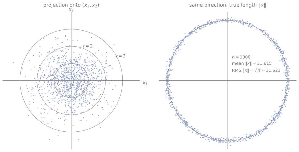
Left figure: Since all of the individual coordinates are independent from each other for a Gaussian, a 2D projection of an $n$-dimensional Gaussian looks, well, exactly like a 2D Gaussian.

Right figure: What we’ve uncovered is that plotting their distances to the center should give us something like a “thin shell”, which is reminiscent of a sphere.

---

What’s more, the variance of this radius is bounded by $\sigma^2$ (again, shown in the appendix): we have

\[\sigma\sqrt{n-1} \le \mathbb{E}[R] \le \sigma\sqrt n,\]

which can be used to bound the variance

\[\mathbb{V}[R] = \mathbb{E}[R^2] - (\mathbb{E}[R])^2 \leq n \sigma^2 - (n-1) \sigma^2 = \sigma^2,\]

which indicates that the variance of the thin shell is actually bounded independent of the dimension $n$.

In fact, we know that the radius of the shell grows like $\sigma\sqrt{n}$, but its spread $\sqrt{\mathbb{V}[R]}$ doesn’t grow at all. Comparing the two we have

\[\frac{\sqrt{\mathbb{V}[R]}}{\mathbb{E}[R]} \le \frac{\sigma}{\sigma\sqrt{n-1}} = \frac{1}{\sqrt{n-1}},\]

so the shell’s thickness relative to its radius shrinks like $1/\sqrt{n}$.

Comparing the ball, the sphere, and the Gaussian

In the volume of the n-ball, we saw how we can uniformly sample from the unit sphere by sampling a vector $\mathbf{v}$ from a multivariate Gaussian and normalizing it with $\mathbf{v} \leftarrow \mathbf{v} / \lVert \mathbf{v} \rVert$ exploiting rotational symmetry. We could also sample from the unit ball as well by scaling the sphere result with $U^{1/n}$.

Let’s uncover more about these three, from the other direction this time.

---

One interesting comparison opportunity arises from comparing the marginal distributions for each of these three objects.

From the volume post, we know that the unit ball $B_{n}$ has a marginal probability of

\[p(t) \propto (1-t^2)^{(n-1)/2},\]

and from the earlier surface post we know the unit sphere $S_{n-1}$ has a marginal probability of

\[p(t) \propto (1-t^2)^{(n-3)/2}.\]

Finally, we know (from this post) that the Gaussian has independent coordinates with marginal probabilities of

\[p(t) = \mathcal{N}(t; 0, \sigma^2).\]

Let’s scale it with $\sigma^2 = \frac{1}{n}$, so that its points form a thin shell around $R = \sigma\sqrt{n} = 1$, just like the boundaries of the ball and sphere.

Here’s how the marginal distributions of the unit $n$-ball and the $(n-1)$-sphere change with increasing dimensionality, compared to a scaled Gaussian with $\sigma^2 = \tfrac1n$:

$n$	$n$-ball	$(n-1)$-sphere	Gaussian
1	uniform on $[-1,1]$	two points: $-1, +1$	$\mathcal{N}(0, \tfrac1n)$
2	semicircle $\sqrt{1-t^2}$	arcsine, $\frac{1}{\sqrt{1-t^2}}$	$\mathcal{N}(0, \tfrac1n)$
3	parabola $1-t^2$	uniform	$\mathcal{N}(0, \tfrac1n)$
large	$\approx \mathcal{N}(0, \tfrac1n)$	$\approx \mathcal{N}(0, \tfrac1n)$	$\mathcal{N}(0, \tfrac1n)$

The uniformly distributed cases of $n=1$ for the ball and $n=3$ for the sphere are quite interesting (the 2-sphere’s uniform distribution is Archimedes’ remarkable hat-box theorem!), however, we see that in the asymptotic case these three all blend into each other.

Of course, the marginal distributions are interesting, however the joint distribution is what uniquely determines the particular distribution. The unit cube and the $2$-sphere both have uniform marginals for $x$, $y$, and $z$, however the sphere’s joint distribution is also constrained by the requirement of $x^2 + y^2 + z^2 = R^2$ for some $R \geq 0$.

This leads us to the unique property of Gaussians, as stated by Herschel-Maxwell’s theorem:

Fun fact! This property was derived from Herschel’s 1850 work on measurements of astronomical star positions, and extended with Maxwell’s 1860 analysis of gas molecule velocities.

---

The important takeaway of the story is that with increasingly larger $n$ (and appropriate scaling), the line between a ball, a sphere, and a (scaled) Gaussian seems to blur into the same thing:

• We saw previously that the volume of the $n$-ball is increasingly concentrated near its boundary, which is the $(n-1)$-sphere.

• We see that the typical point of a Gaussian concentrates again on a thin shell around $\sigma\sqrt{n}$, which resembles a sphere of radius $\sigma\sqrt{n}$.

---

Closing remarks

There is obviously so much more about Gaussians in high dimensional space, but I think this is a good point to finish the post in terms of length. I might revisit this topic again soon though.

I think the next post will be on distances and angles. It will probably start off from the very famous property of near-orthogonality of random vectors, and will continue from our Gaussian discussion:

---

Appendix

Deriving $\mathbb{E}[R]$

Throughout this section we have $X \sim \mathcal{N}(0, \sigma^2 I_n)$ and $R = \lVert X \rVert$. Claude was a huge help in the main idea and the heavier math parts.

The idea is to find the distribution of $R$, and then compute the moments of $R$. $\mathbb{E}[R^m]$ is called the $m$-th (raw) moment of $R$, and we’ll use the first and second raw moments to find $\mathbb{E}[R]$ and $\mathbb{V}[R]$.

We’ll proceed in a series of steps.

Step 1: the distribution of the radius via the onion method

How is $R$ distributed? Since the Gaussian is unbounded, technically any radius is possible. We’re going to use the same onion method from the surface post.

---

The density of the isotropic Gaussian only depends on $\mathbf{x}$ through its length $r = \lVert \mathbf{x} \rVert$:

\[p(\mathbf{x}) = \frac{1}{(2\pi\sigma^2)^{n/2}}\,e^{-\lVert \mathbf{x} \rVert^2/2\sigma^2}.\]

So the density is constant on every sphere centered at the origin, and we can slice $\mathbb{R}^n$ into onion layers, just like in the surface post. The probability of landing in the thin shell between $r$ and $(r + dr)$ is the density on that shell multiplied by the shell’s volume, $S_{n-1}(r)\,dr$:

\[P(r \le R \le r + dr) \approx p(\mathbf{x})\Big|_{\lVert \mathbf{x} \rVert = r} \cdot S_{n-1}(r)\,dr.\]

Using $S_{n-1}(r) = \frac{2\pi^{n/2}}{\Gamma(n/2)}r^{n-1}$, the density of $R$ is

\[\begin{align} p_R(r) &= \frac{2\pi^{n/2}}{\Gamma(n/2)}\,r^{n-1}\cdot\frac{1}{(2\pi\sigma^2)^{n/2}}\,e^{-r^2/2\sigma^2} \\ &= \frac{2}{(2\sigma^2)^{n/2}\,\Gamma(n/2)}\,r^{n-1}\,e^{-r^2/2\sigma^2}, \qquad r \ge 0. \tag{A1} \label{eq:radial} \end{align}\]

Conceptually, the two factors pull in opposite directions: $r^{n-1}$ (the sphere getting bigger) pushes the mass outwards, while $e^{-r^2/2\sigma^2}$ (the Gaussian) pulls it back in. The thin shell is where these two balance out.

Step 2: one integral for every moment

Every moment $\mathbb{E}[R^m]$ needs an integral of the form $\int_0^\infty r^k e^{-r^2/2\sigma^2}\,dr$, so let’s do it once. Recall that the Gamma function is defined by

\[\Gamma(z) = \int_0^\infty t^{z-1}e^{-t}\,dt, \qquad z > 0.\]

We have

\[\int_0^\infty r^k e^{-r^2/2\sigma^2}\,dr = \frac{1}{2}(2\sigma^2)^{(k+1)/2}\,\Gamma\!\left(\frac{k+1}{2}\right). \tag{A2} \label{eq:gammaint}\]

Why is the integral a Gamma function?

Substitute $t = r^2/2\sigma^2$, so that

\[r = (2\sigma^2 t)^{1/2}, \qquad dr = \frac{1}{2}(2\sigma^2)^{1/2}\,t^{-1/2}\,dt.\]

Then

\[\begin{align} \int_0^\infty r^k e^{-r^2/2\sigma^2}\,dr &= \int_0^\infty (2\sigma^2 t)^{k/2}\,e^{-t}\cdot\frac{1}{2}(2\sigma^2)^{1/2}\,t^{-1/2}\,dt \\ &= \frac{1}{2}(2\sigma^2)^{(k+1)/2}\int_0^\infty t^{(k-1)/2}e^{-t}\,dt \\ &= \frac{1}{2}(2\sigma^2)^{(k+1)/2}\,\Gamma\!\left(\tfrac{k+1}{2}\right). \end{align}\]

Now the $m$-th moment of $R$ is \eqref{eq:radial} multiplied by $r^m$, i.e. \eqref{eq:gammaint} with $k = n - 1 + m$:

\[\begin{align} \mathbb{E}[R^m] &= \frac{2}{(2\sigma^2)^{n/2}\,\Gamma(n/2)}\int_0^\infty r^{n-1+m}e^{-r^2/2\sigma^2}\,dr \\ &= \frac{2}{(2\sigma^2)^{n/2}\,\Gamma(n/2)}\cdot\frac{1}{2}(2\sigma^2)^{(n+m)/2}\,\Gamma\!\left(\frac{n+m}{2}\right) \\ &= (2\sigma^2)^{m/2}\,\frac{\Gamma\!\left(\frac{n+m}{2}\right)}{\Gamma\!\left(\frac{n}{2}\right)}. \tag{A3} \label{eq:moments} \end{align}\]

Let’s do a sanity check on \eqref{eq:moments} with two values before using it:

• $m = 0$ gives $\mathbb{E}[1] = \Gamma(n/2)/\Gamma(n/2) = 1$, so $p_R$ integrates to $1$ as a density should.
• $m = 2$ gives $2\sigma^2\cdot\Gamma(\frac{n}{2} + 1)/\Gamma(\frac{n}{2}) = 2\sigma^2\cdot\frac{n}{2} = n\sigma^2$ using $\Gamma(z+1) = z\Gamma(z)$, which matches the RMS result $\mathbb{E}[R^2] = n\sigma^2$ from the main text.

Step 3: the expected radius

With $m = 1$ we get our result:

\[\boxed{\mathbb{E}[R] = \sigma\sqrt{2}\,\frac{\Gamma\!\left(\frac{n+1}{2}\right)}{\Gamma\!\left(\frac{n}{2}\right)}}. \tag*{$\Box$}\]

For $n = 1$, $\Gamma(1) = 1$ and $\Gamma(\frac{1}{2}) = \sqrt{\pi}$ give $\sqrt{2/\pi}\,\sigma$, the mean absolute distance from the 1D case.

Bounding $\mathbb{E}[R]$ and $\mathbb{V}[R]$

We now show that

\[\sigma\sqrt{n-1} \;\le\; \mathbb{E}[R] \;\le\; \sigma\sqrt{n}.\]

In the appendix of the surface post, we defined

\[g(x) = \frac{\Gamma(x+1)}{\Gamma(x+\frac{1}{2})}\]

and showed with the squeeze theorem that for $x > 0$,

\[\sqrt{x} \le g(x) \le \sqrt{x + \tfrac{1}{2}}.\]

The Gamma ratio in $\mathbb{E}[R]$ is exactly $g$ in disguise: setting $x = \frac{n-1}{2}$ gives $x + 1 = \frac{n+1}{2}$ and $x + \frac{1}{2} = \frac{n}{2}$, so

\[\mathbb{E}[R] = \sigma\sqrt{2}\cdot g\!\left(\tfrac{n-1}{2}\right).\]

Applying the bounds for $n \ge 2$:

\[\sigma\sqrt{2}\cdot\sqrt{\frac{n-1}{2}} \;\le\; \mathbb{E}[R] \;\le\; \sigma\sqrt{2}\cdot\sqrt{\frac{n}{2}} \qquad\Longrightarrow\qquad \sigma\sqrt{n-1} \;\le\; \mathbb{E}[R] \;\le\; \sigma\sqrt{n}.\]

The case $n = 1$ can be checked directly, since $0 \le \sqrt{2/\pi}\,\sigma \approx 0.798\,\sigma \le \sigma$. $\Box$

---

We can now follow this up with the variance bound. Using $\mathbb{E}[R^2] = n\sigma^2$ and the lower bound on $\mathbb{E}[R]$,

\[\mathbb{V}[R] = \mathbb{E}[R^2] - (\mathbb{E}[R])^2 \le n\sigma^2 - (n-1)\sigma^2 = \sigma^2. \tag*{$\Box$}\]